Introduction
Divvy is a bike sharing system for the city of Chicago that provides residents and tourists an option for getting around the city. After patrons purchase a daily or annual pass, they can unlock a bike, ride to their destination, and return the bike to one of the Divvy bike docking stations found throughout the city. The daily and annual pass includes 30 minutes of riding time, with additional fees for longer trips. The program is designed to promote short one-way trips to increase sharing of the bikes throughout the day. The program currently has 6,000 bikes at over 580 bike stations and there are similar bike sharing programs in other cities, including Montreal and Boston.
The motivation to forecast Divvy bike use would be beneficial for Divvy’s operating company, Motivate, and the Chicago Department of Transportation for the following reasons.
- Predicting the demand for the next season would aid plans on future expansion or price changes to opimize bike use and profitability.
- On a granular level, identifying the patterns of use for each bike station would allow the Divvy program to opimize bike placement and availability. Stations that are predicted to have increasing use can be expanded for additional Divvy bike slots, and it may be necessary to transport bikes from one station to another.
- The Divvy program can be used as a measure of transportation activity in the city and can tell us how people move about the city on a day-to-day and week-to-week basis.
Exploring the Divvy data
This project will attempt to model the daily duration of Divvy rides for all bike stations in the city. The data was collected from the City of Chicago Data Portal. The original data was summarized using the Data Portal Filter by summing the daily duration of each trip, and then exported to a csv file. The summarized data is public and available here. The duration is total hours of bike usage per day.
library(tidyverse)
library(lubridate)
library(forecast)
library(knitr)
library(xts)

divvy <- read_csv("divvy_daily_duration.csv")

divvy$date <- mdy(divvy$`START TIME`)
divvy$`START TIME` <- NULL
divvy$duration <- divvy$`TRIP DURATION`
divvy$`TRIP DURATION` <- NULL
First we will look at the overall time series and examine its features.
divvy_xts <- xts(divvy$duration, order.by = divvy$date)
fig1 <- autoplot(divvy_xts) + ggtitle("Divvy daily ridership duration") + ylab("Hours per day") + xlab("Year")
fig1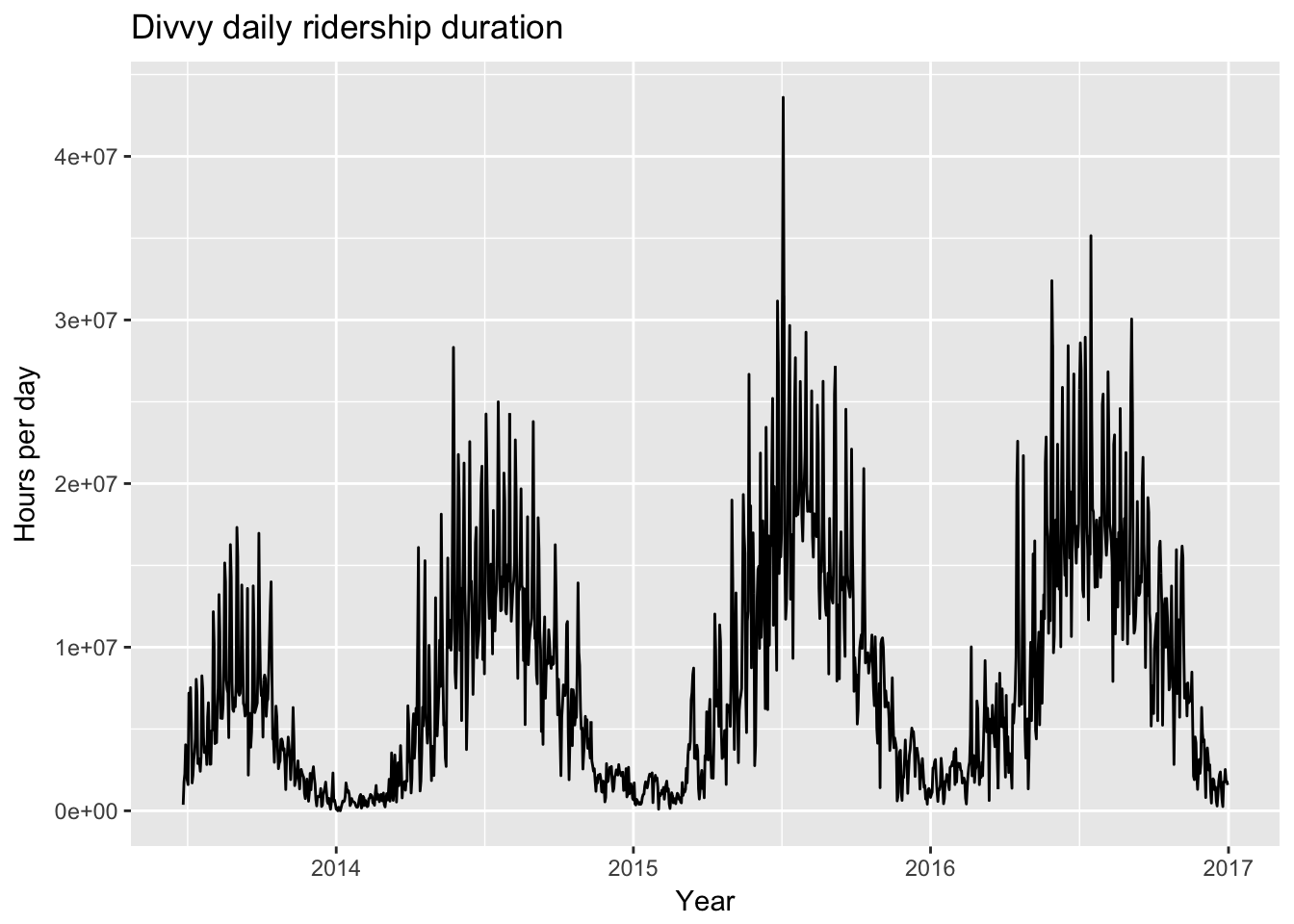
(#fig:Time series plot)Divvy Bike Time Series
We can see that ridership appears to have increased during the first three years of Divvy availability and possibly leveled off during 2016, the last year of available data. There is also clear yearly seasonality, which is expected given how difficult it is to ride a bicycle during Chicago’s winters.
divvy_ts <- ts(divvy_xts, start = c(2013, 178), frequency = 365)
fig2 <- ggseasonplot(divvy_ts) + ggtitle("Seasonal plot of Divvy daily ridership")
fig2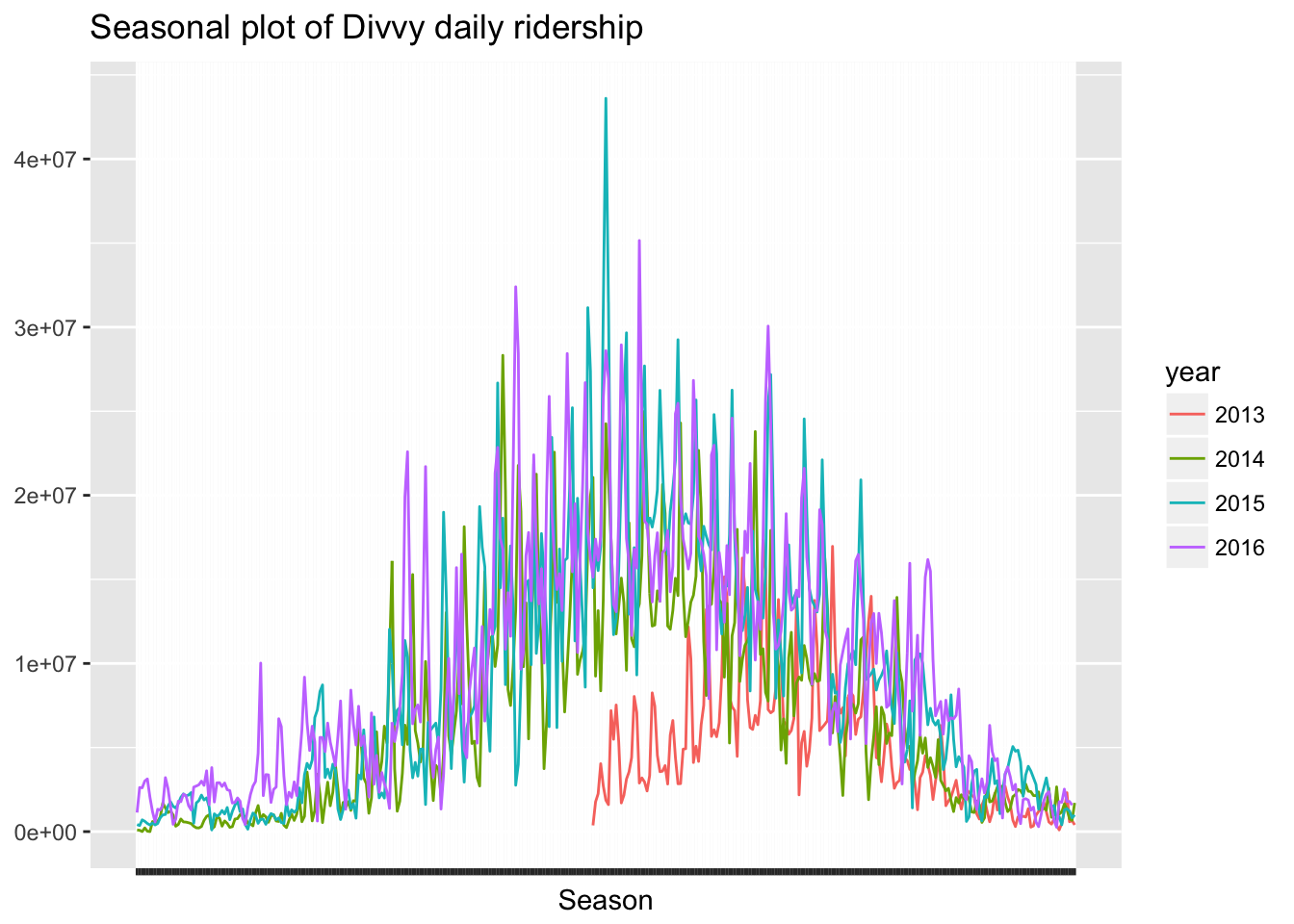
The first year of the Divvy program seems to have started slowly in the summer of 2013 and since then, summer has been a much more actively used time for the program. For this reason I will be only using 2014-2016 data.
divvy_ts <- ts(divvy_xts, start = c(2014, 1), frequency = 365)
divvy_xts <- divvy_xts['2014/2017']
divvy <- filter(divvy, date >= "2014-01-01")
Since Divvy is used by many commuters, its possible there is also weekly seasonality as well. However, let’t take a closer look at 4 weeks of data in May 2016.
plot(divvy_xts['2016-05-01/2016-05-28'])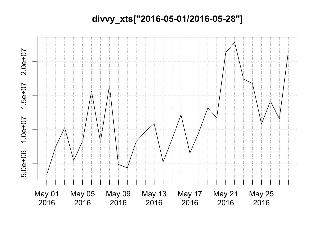
During this time, there doesn’t appear to be any obvious weekly seasonality to the data. We can also examine the subseries plot for each week day over all years.
divvy_w_ts <- ts(divvy_xts['2014-01-01/2016-12-31'], start = c(2014, 1), frequency = 7)
fig3 <- ggsubseriesplot(divvy_w_ts) + ggtitle("Subseries plot for weekly seasonality")
fig3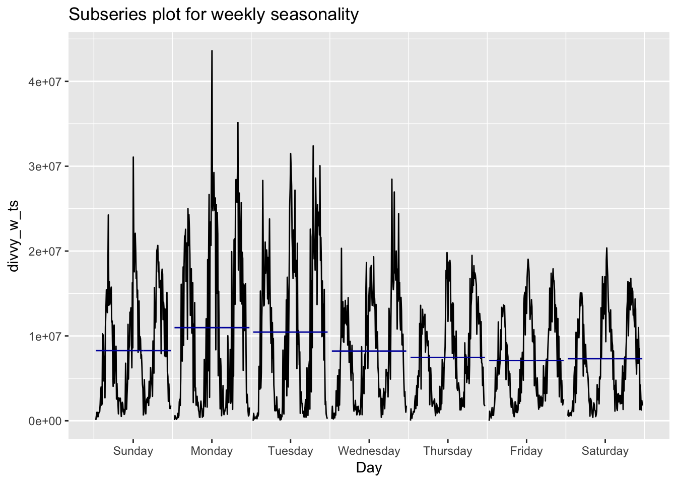
This does look like there is some seasonality with the highest volume of traffic on Monday’s and Tuesdays.
To explore annual trends we can combine the data into a weekly and monthly series.
divvy_w <- divvy %>% group_by(week = as.POSIXct(cut(date, "week"))) %>% summarise(weekly_rides = sum(duration))
divvy_m <- divvy %>% group_by(month = as.POSIXct(cut(date, "month"))) %>% summarise(monthly_rides = sum(duration))
Let’s split out the latter half of 2016 as a test set so that we can examine how well our models forecast future Divvy bike rider duration.
divvy_d_test <- divvy_xts['2016-07-01/2016-12-31']
divvy_w_test <- divvy_w %>% filter(week >= "2016-07-01")
divvy_m_test <- divvy_m %>% filter(month >= "2016-07-01")

divvy_d_train <- divvy_xts['2014/2016-07-01']
divvy_w_train <- divvy_w %>% filter(week < "2016-07-01")
divvy_m_train <- divvy_m %>% filter(month < "2016-07-01")

divvy_m_train <- xts(divvy_m_train$monthly_rides, order.by = divvy_m_train$month)
Modeling monthly
Let’s first try modeling the longer term series with monthly data, first with an auto ETS damped model.
d_ts <- ts(divvy_m_train, start = 2014, frequency = 12)
fit1 <- ets(d_ts, damped = TRUE)
summary(fit1)
## ETS(A,Ad,N)
##
## Call:
## ets(y = d_ts, damped = TRUE)
##
## Smoothing parameters:
## alpha = 0.9711
## beta = 0.9706
## phi = 0.8
##
## Initial states:
## l = 20635973.97
## b = 39426295.083
##
## sigma: 69894089
##
## AIC AICc BIC
## 1197.785 1201.438 1206.193
##
## Training set error measures:
## ME RMSE MAE MPE MAPE MASE
## Training set 6168957 69894089 51645030 7.894976 35.8655 0.8955505
## ACF1
## Training set 0.1098338fig4 <- autoplot(forecast(fit1, h = 6))
fig4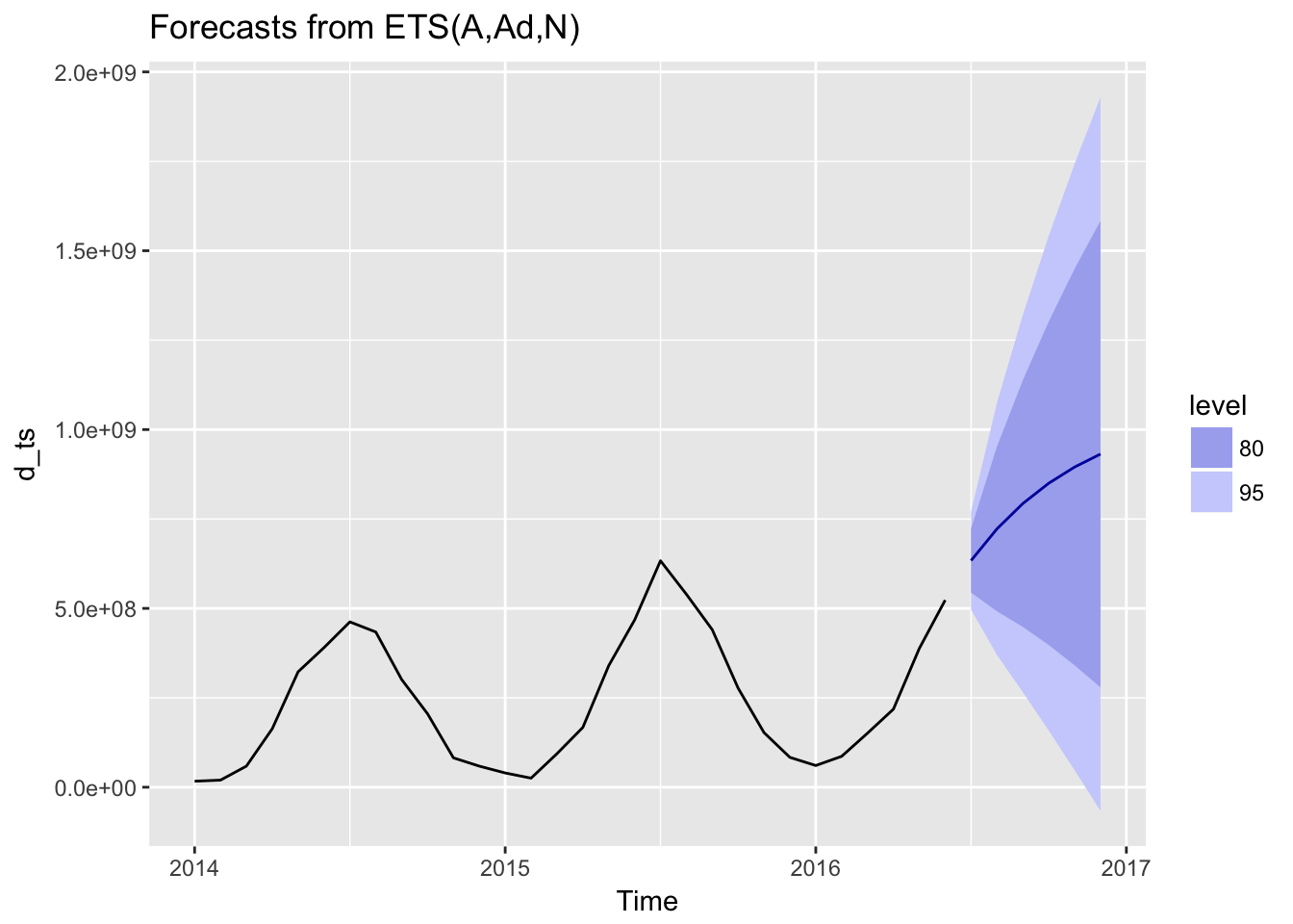
This does not appear to be a good forecast, since there is no accounting for seasonality.
?ets
fit1b <- ets(d_ts, model = c("AAA"), damped = TRUE)
summary(fit1b)
## ETS(A,Ad,A)
##
## Call:
## ets(y = d_ts, model = c("AAA"), damped = TRUE)
##
## Smoothing parameters:
## alpha = 0.0755
## beta = 1e-04
## gamma = 0.9244
## phi = 0.98
##
## Initial states:
## l = 193446765.697
## b = 5152994.1269
## s=-179142977 -152246416 -25321253 78782509 210768148 261071506
## 174544061 110759629 -44819085 -145723334 -181035730 -107637058
##
## sigma: 38103138
##
## AIC AICc BIC
## 1185.384 1247.566 1210.606
##
## Training set error measures:
## ME RMSE MAE MPE MAPE MASE
## Training set 753174.4 38103138 23033648 -24.60122 31.12008 0.3994149
## ACF1
## Training set 0.50219fc1 <- forecast(fit1b, h = 6)
plot(fc1, showgap = FALSE)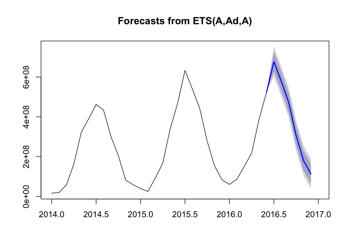
This is much better, since our seasonality has a very large effect on the overall series.
Arima
Next, we will try exploring a seasonal Arima model. First, let’s look at the ACF and PACF plots on the orininal series.
ggtsdisplay(divvy_m_train, main="Monthly Divvy Usage")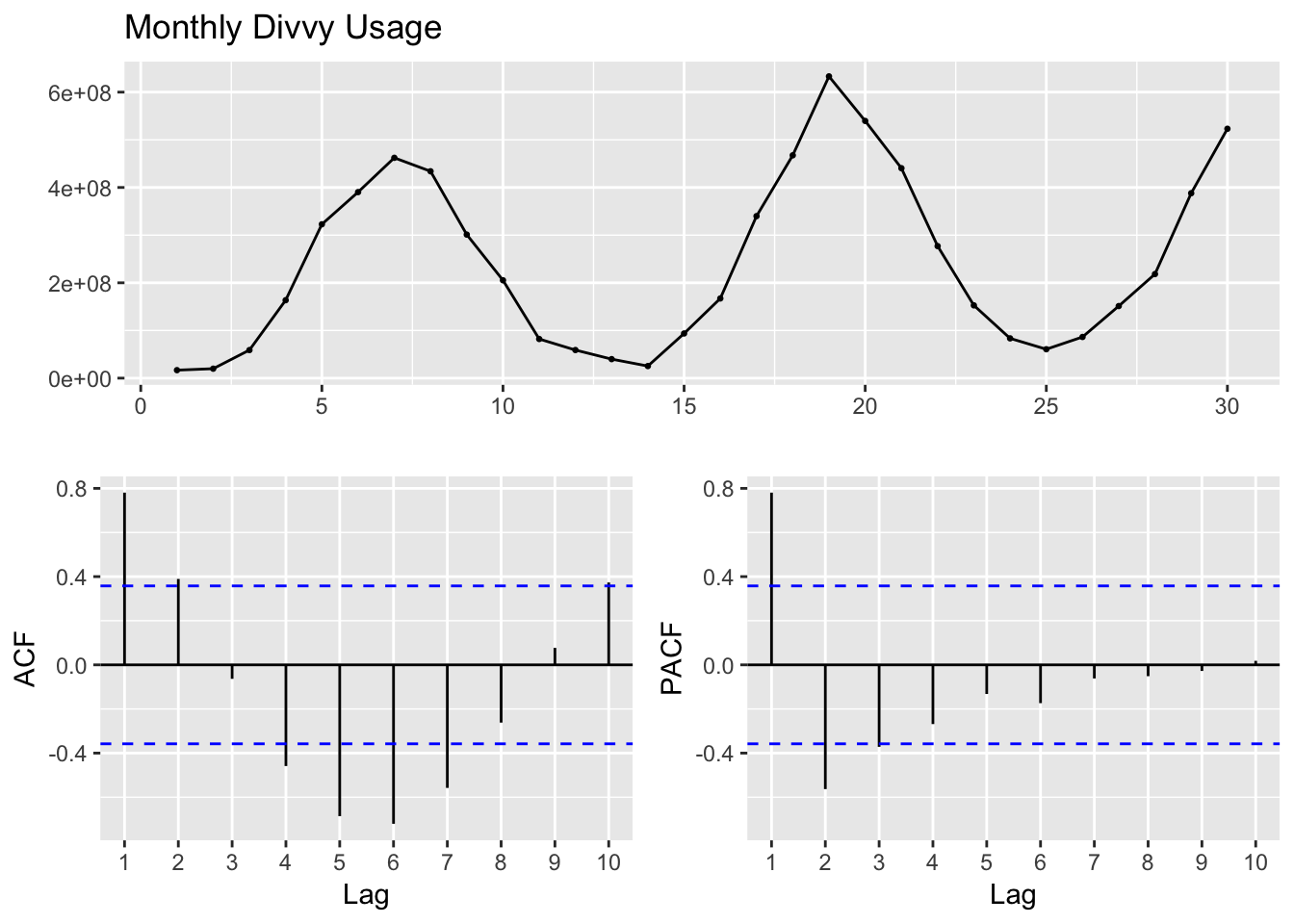
This series is not stationary, in part because of the seasonality. Next I’ll examine a differenced series with a lag of 12 to remove the seasonality and determine whether that is stationary.
ggtsdisplay(diff(divvy_m_train, lag = 12))## Warning: Removed 12 rows containing missing values (geom_point).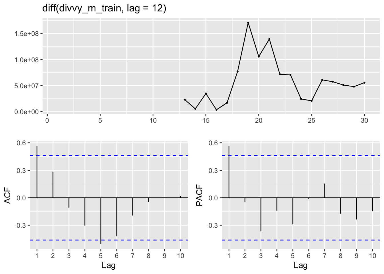
The PACF indicates that there is still autocorrelation from the previous lag. Taking a second difference with a lag of 1 should result in stationary series.
ggtsdisplay(diff(diff(divvy_m_train, lag = 12)))## Warning: Removed 13 rows containing missing values (geom_point).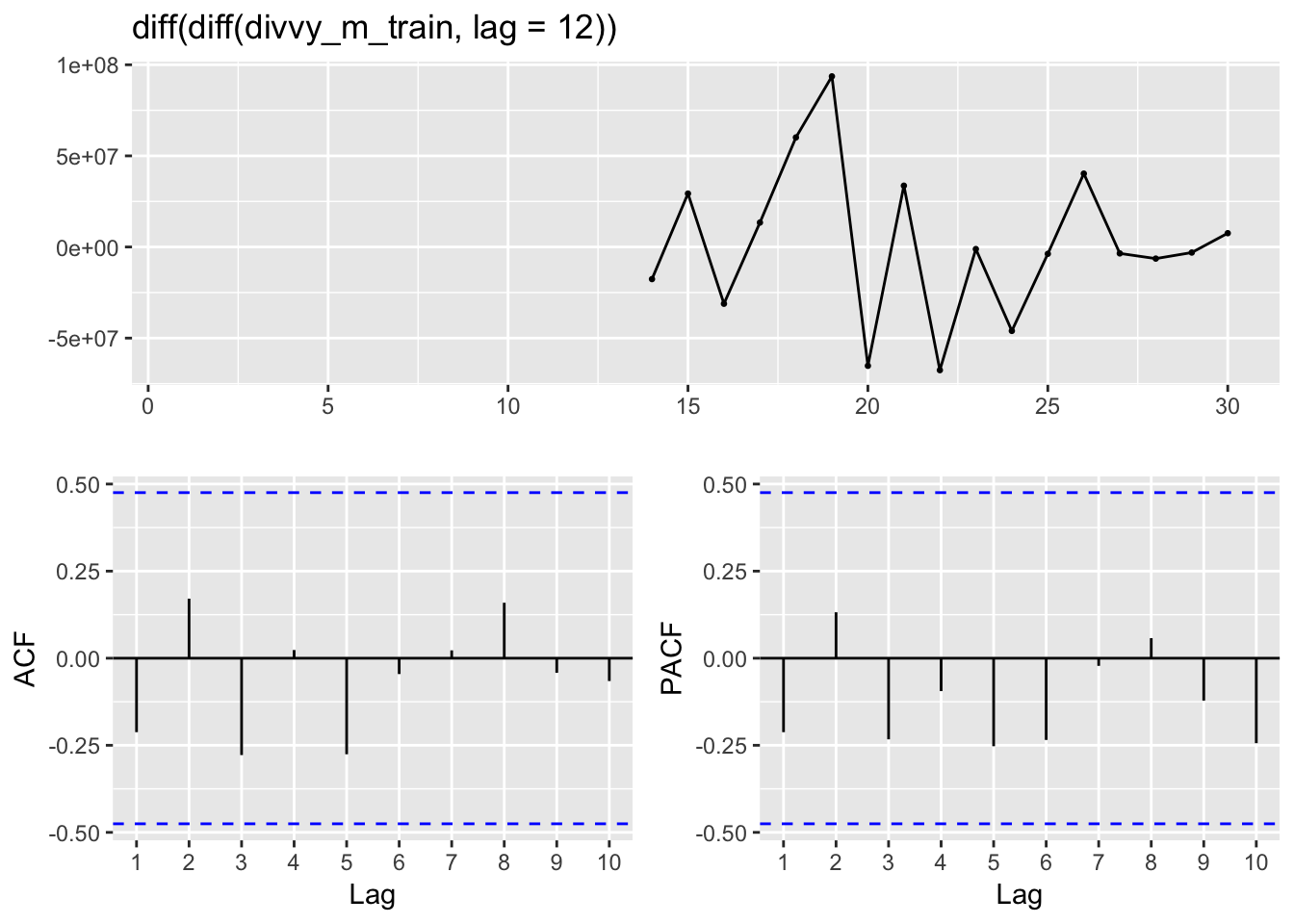
Indeed, this now appears to be a stationary time series. This indicates we should model the series with an ARIMA with a nonseasonal differencing of 1 and a seasonal differencing of 12.
fit2 <- Arima(divvy_m_train, order = c(0,1,1), seasonal = list(order = c(0,1,1), period = 12))
fit3 <- Arima(divvy_m_train, order = c(0,1,0), seasonal = list(order = c(0,1,1), period = 12))
fit4 <- Arima(divvy_m_train, order = c(0,1,1), seasonal = list(order = c(0,1,0), period = 12))
fit5 <- Arima(divvy_m_train, order = c(1,1,0), seasonal = list(order = c(0,1,0), period = 12))
fit6 <- Arima(divvy_m_train, order = c(2,1,0), seasonal = list(order = c(0,1,1), period = 12))
fit7 <- Arima(divvy_m_train, order = c(2,1,0), seasonal = list(order = c(0,1,2), period = 12))


arima_comp <- data.frame(ARIMA = c("(0,1,1)(0,1,1)12",
                                   "(0,1,0)(0,1,1)12",
                                   "(0,1,1)(0,1,0)12",
                                   "(1,1,0)(0,1,0)12",
                                   "(2,1,0)(0,1,1)12",
                                   "(2,1,0)(0,1,2)12"),
                         AIC = c(fit2$aic, fit3$aic, fit4$aic, fit5$aic, fit6$aic, fit7$aic))
save(arima_comp, file = "arima_comp.RData")
kable(arima_comp)| ARIMA | AIC |
|---|---|
| (0,1,1)(0,1,1)12 | 649.5367 |
| (0,1,0)(0,1,1)12 | 648.0710 |
| (0,1,1)(0,1,0)12 | 647.6083 |
| (1,1,0)(0,1,0)12 | 647.4803 |
| (2,1,0)(0,1,1)12 | 651.0671 |
| (2,1,0)(0,1,2)12 | 653.0670 |
The Arima model with the lowest AIC is an \(ARIMA(1,1,0)(0,1,0)_{12}\)
fc5 <- forecast(fit5, h=6)
plot(fc5, showgap = FALSE)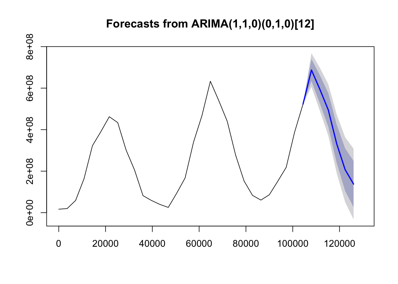
Prophet
I wanted to try out the new dynamic regression forecasting tool published by Facebook, called Prophet. It’s very easy to create a model using the Prophet package as there are very few parameters that you need to set.
library(prophet)## Loading required package: Rcppdivvy_m_prophet <- data.frame(ds = divvy_m$month, y = divvy_m$monthly_rides)
divvy_m_prophet <- divvy_m_prophet %>% filter(ds < "2016-07-01")
m <- prophet(divvy_m_prophet)## Warning in set_auto_seasonalities(m): Disabling weekly seasonality. Run
## prophet with `weekly.seasonality=TRUE` to override this.## Initial log joint probability = -3.6839
## Optimization terminated normally:
## Convergence detected: absolute parameter change was below tolerancefuture <- make_future_dataframe(m, periods = 6, freq = 'month')
fc6 <- predict(m, future)
plot(m, fc6)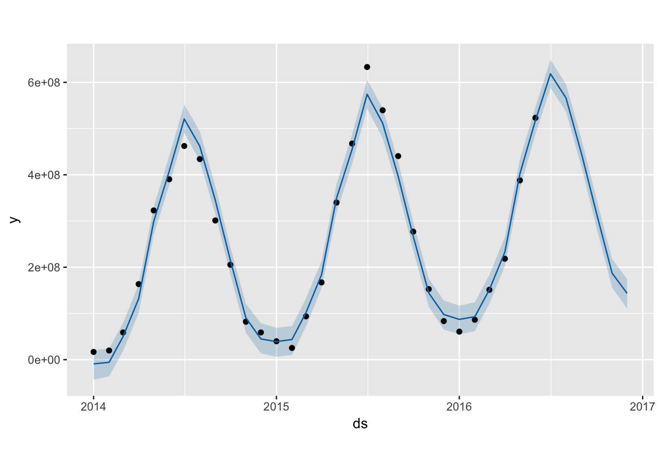
Model comparison
mo_comp <- data.frame(actual = divvy_m_test$monthly_rides, ets = fc1$mean, arima = fc5$mean, prophet = tail(fc6$yhat))

ets_sse <- with(mo_comp, expr = sum((actual - ets)^2))
arima_sse <- with(mo_comp, expr = sum((actual - arima)^2))
prophet_sse <- with(mo_comp, expr = sum((actual - prophet)^2))
mo_comp <- data.frame(Model = c("TBATS", "ARIMA", "Prophet"), "SSE" = c(ets_sse, arima_sse, prophet_sse))

kable(mo_comp)| Model | SSE |
|---|---|
| TBATS | 1.386430e+16 |
| ARIMA | 2.223434e+16 |
| Prophet | 9.838822e+15 |
The prophet model has a lower SSE than the ets(A,Ad,A) model, which has a lower error rate than the \(ARIMA(1,1,0)(0,1,0)_{12}\). These forecasts might be useful for longer term trends, perhaps for planning on year-to-year changes. However, for more granular predictions, we need to explore the daily time series data.
Modeling daily Divvy durration within the year
Combined ETS + ARMA for double seasonal modeling
Since the daily time series data have both a weekly and yearly seasonality, we need to use the msts function to specify our multiple seasons. We can then use a modeling method that will work with such multiple seasonality time series, such as a the tbats function for exponential smoothing.
divvy_d_msts <- msts(divvy_d_train, seasonal.periods = c(7, 365.25))
fit11 <- tbats(divvy_d_msts)
fc11 <- forecast(fit11, h=184)
plot(fc11)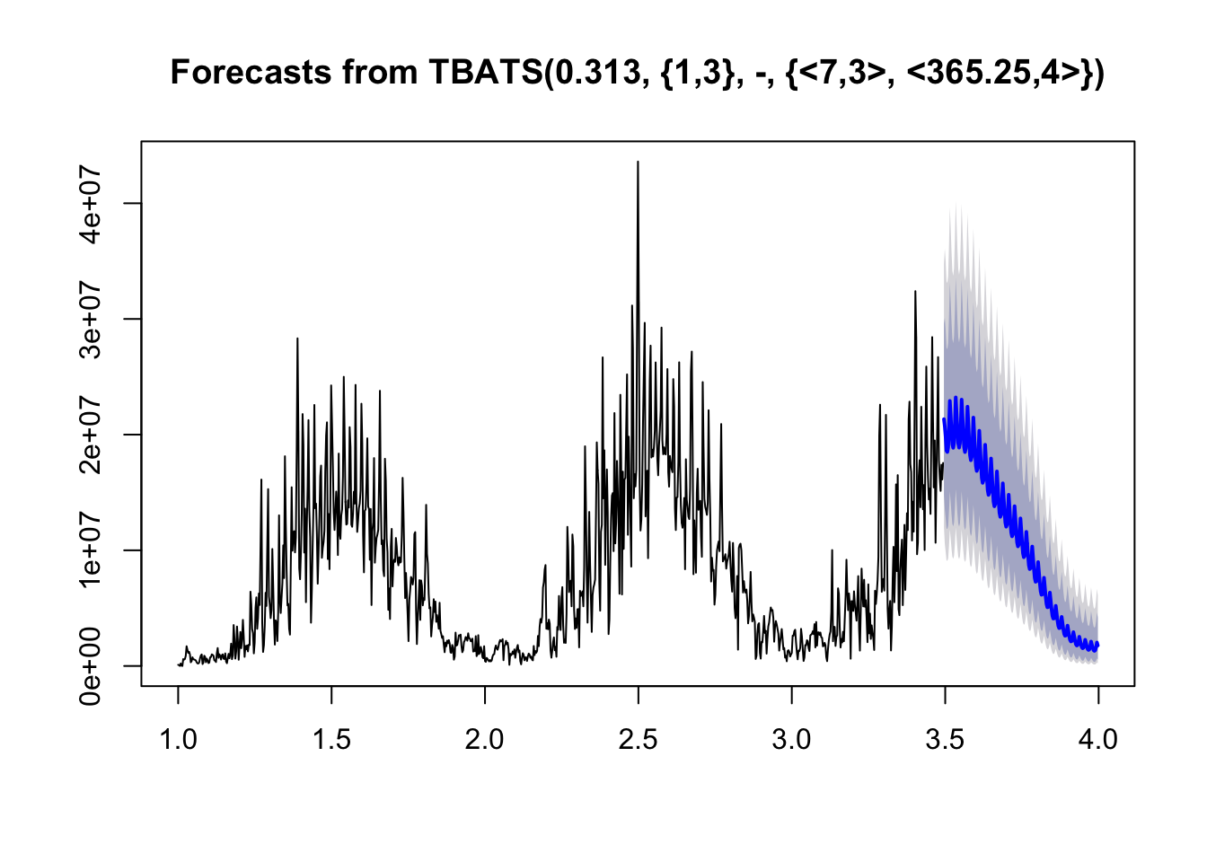
This forecast looks quite good, especially how the predicted variance scales down as the predicted point values drop, which matches the variance in the time series.
I am not aware of any ARIMA based methods that will work for complex seasonality, so next up is building a Prophet model.
Prophet daily
divvy_d_prophet <- data.frame(ds = divvy$date, y = divvy$duration)
divvy_d_prophet_train <- divvy_d_prophet %>% filter(ds < "2016-07-01")

d <- prophet(divvy_d_prophet_train)
## Initial log joint probability = -16.0823
## Optimization terminated normally:
## Convergence detected: relative gradient magnitude is below tolerancefuture <- make_future_dataframe(d, periods = 184)
fc13 <- predict(d, future)
plot(d, fc13)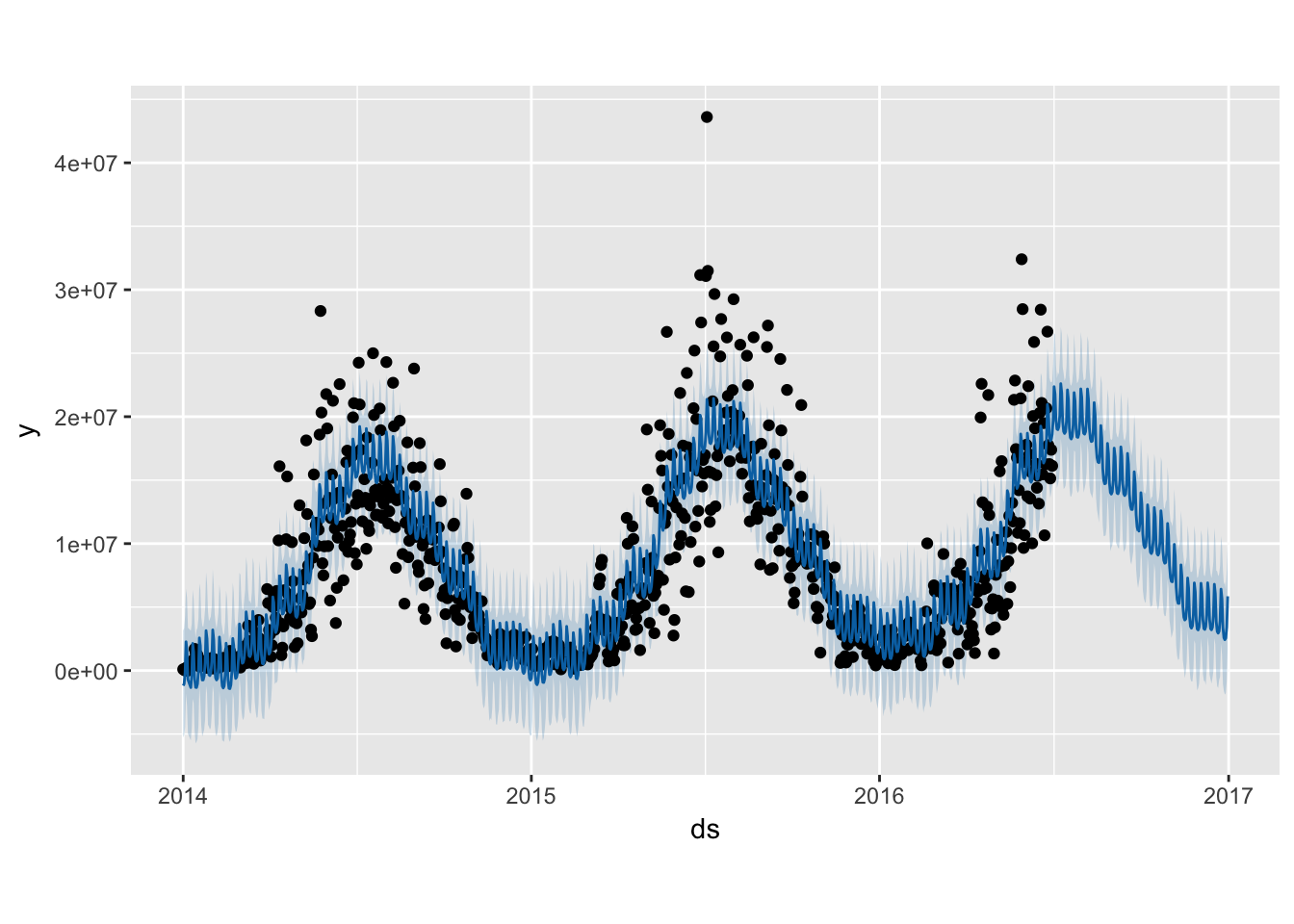
prophet_plot_components(d, fc13)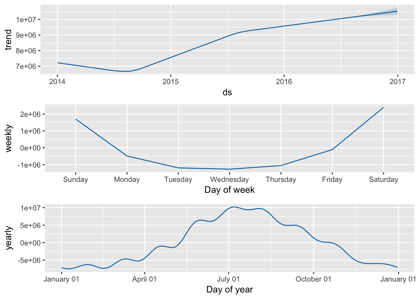
Interestingly, the prophet package interprets our weekly seasonality as having higher demand on the weekends, which makes more intuitive sense. There might be an issue with how I defined the ts object and how it defines days of the weeks. While this potential ‘bug’ might affect our inference for the effect that any particular day of the week has on the estimate, it should not impact our overall forecasting ability.
The Prophet model does not seem to show changing variance from summer to winter as the TBATS model did.
Model comparison and selection
comparison <- data.frame(actual = divvy_d_test, tbats = fc11$mean, prophet = tail(fc13$yhat, 184))

tbats_sse <- with(comparison, expr = sum((actual - tbats)^2))
prophet_sse <- with(comparison, expr = sum((actual - prophet)^2))

tbats_sse_1mo <- with(comparison[1:30,], expr = sum((actual - tbats)^2))
prophet_sse_1mo <- with(comparison[1:30,], expr = sum((actual - prophet)^2))

comp <- data.frame(Model = c("TBATS", "Prophet"), "SSE.1Mo" = c(tbats_sse_1mo, prophet_sse_1mo), "SSE.6Mo" = c(tbats_sse, prophet_sse))

kable(comp)| Model | SSE.1Mo | SSE.6Mo |
|---|---|---|
| TBATS | 9.629984e+14 | 3.481454e+15 |
| Prophet | 6.540232e+14 | 2.559338e+15 |
The Prophet model beats the TBATS model for both short (1-Month) estimates and longer term (6 month) estimates. These two models both incorporate the weekly and annual seasonality of the data. The Prophet model also seems to show an additional fluxuation to the fitted pattern that is not quite a monthly seasonality but very close.
Conclusion and future improvements
The double seasonality of the Divvy data set required the use of advanced time series forecasting approaches, and precluded the use of simple exponential smoothing and autoregressive models. The new forecasting tool Prophet, created by Facebook, performs better than the TBATS function, from the Forecast package, in both short term and long term predictions. It also was the top model for long term monthly data as well.
One additional feature that can be added to the Prophet model is the effect of specific holidays. The highest demand day in the data set was on July 4, 2015, a holiday which also fell on a Saturday. Other years had very high demand during the days around Independence Day as well, and this effect could be included in the model. Weather variables could also be incorporated into the model, such as temperature and precipitation. However, weather is not generally known far in advance and including those features might have limited forecasting potential.